Different methods of generating qqplot
The Q-Q plot, also known as the quantile-quantile plot, is a graphical tool that helps us determine whether a set of data originated from a Normal or exponential distribution. For instance, if a statistical analysis assumes that residuals are normally distributed, a Normal Q-Q plot can be used to verify this assumption. This is merely a visual inspection and not a conclusive proof, so it is somewhat subjective. However, it enables us to see at a glance whether our assumption is plausible, and if not, how the assumption is violated and which data points contribute to the violation. A Q-Q plot is a scatterplot created by superimposing two quantile distributions. If both sets of quantiles came from the same distribution, the points should form a roughly straight line.
This post focuses primarily on introducing functions that can reproduce the Q-Q plot.
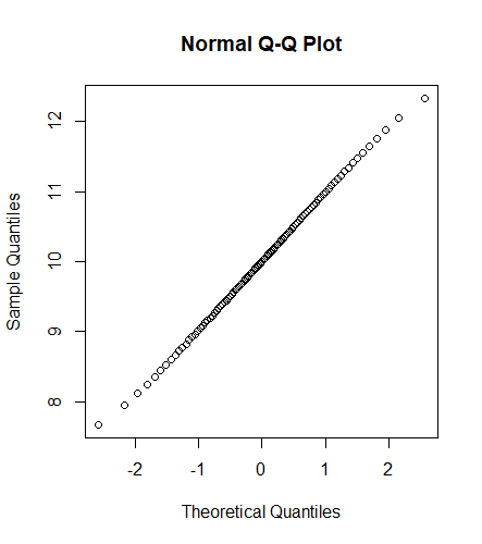
qqnormis a generic function whose default method generates a standard QQ plot of the y values.
1 | > # generate points from normal distribution |
This can be reproduced using the function ppoints, which generates the sequence of probability points, as follows:
1 | > # generate points from normal distribution |

qqplot could also reproduce the above
1 | > # generate points from normal distribution |
qplot could also reproduce the above
1 | > library(ggplot2) |

For residual plot, however, we may choose to plot standardized residuals against theoretical quantiles in Q-Q plot.
We can use the R dataset randu as an illustration.
1 | > str(randu) |
- If dependent variable is scaled, normal residual qqplot could be different
1 | > model <- lm(z ~x+y, data = randu) |

Clearly, scaling the dependent variable z affects the residual.
Before scaling
1 | > model <- lm(z ~x+y,data = randu) |
After scaling
1 | > model <- lm(10*z~x+y,data =randu) |
Using standardized residuals, the expected value of the residuals is zero, while the variance is (approximately) one. This has two benefits:
- If you rescale one of your variables, the residual plots will not change.
- The residuals in the qqplot should lie on the line y = x
- The residuals in the qqplot should lie on the line y = x You anticipate that 95% of your residuals will fall between -1.96 and 1.96. This makes it simpler to identify outliers.
1 | > model <- lm(z ~x+y,data = randu) |
