0%

chi2 is mainly used for binary indicator or term counts, so one needs to be really careful when doing Pearson chi-square test. I will provide several functions to compare these differences, the dataset which I use is the pima dataset

A peek of the dataset

1
2
3
4
5
6
7
8
from pandas import read_csv

# load data
filename = 'dataset/diabetes.csv'
names = ['preg', 'plas', 'pres', 'skin', 'test', 'mass', 'pedi', 'age', 'class']
dataframe = read_csv(filename)
dataframe.columns = names
dataframe.head(2)
preg plas pres skin test mass pedi age class
0 6 148 72 35 0 33.6 0.627 50 1
1 1 85 66 29 0 26.6 0.351 31 0

Use function chi2

  • Convert data frame to the array
1
2
array = dataframe.values
array
1
2
3
4
5
6
7
array([[  6.   , 148.   ,  72.   , ...,   0.627,  50.   ,   1.   ],
[ 1. , 85. , 66. , ..., 0.351, 31. , 0. ],
[ 8. , 183. , 64. , ..., 0.672, 32. , 1. ],
...,
[ 5. , 121. , 72. , ..., 0.245, 30. , 0. ],
[ 1. , 126. , 60. , ..., 0.349, 47. , 1. ],
[ 1. , 93. , 70. , ..., 0.315, 23. , 0. ]])
  • Use chi2 to calculate chi-square values
1
2
3
4
5
6
7
import pandas as pd
from sklearn.feature_selection import chi2

# chi square values
scores,pvalues = chi2(X,Y)
scores
pd.Series(scores,index = names[0:8])
1
2
3
4
5
6
7
8
9
preg     111.519691
plas 1411.887041
pres 17.605373
skin 53.108040
test 2175.565273
mass 127.669343
pedi 5.392682
age 181.303689
dtype: float64

Accumulate values under the same class

1
2
3
4
5
6
7
8
9
10
11
12
13
14
15
16
17
18
19
20
21
22
23
24
25
26
27
28
29
30
31
32
33
# %%
import pandas as pd
import numpy as np
from scipy.sparse import issparse
from sklearn.utils import check_array
from sklearn.preprocessing import LabelBinarizer
from sklearn.utils.extmath import safe_sparse_dot

label = 'class'
X,y = dataframe.drop(columns = label), dataframe[label]

def preprocess_X_y(X, y):
X = check_array(X, accept_sparse="csr")
if np.any((X.data if issparse(X) else X) < 0):
raise ValueError("Input X must be non-negative.")

Y = LabelBinarizer().fit_transform(y)
if Y.shape[1] == 1:
Y = np.append(1 - Y, Y, axis=1)

observed = safe_sparse_dot(Y.T, X) # n_classes * n_features

feature_count = X.sum(axis=0).reshape(1, -1)
class_prob = Y.mean(axis=0).reshape(1, -1)
expected = np.dot(class_prob.T, feature_count)
return observed, expected

f_obs, f_exp = preprocess_X_y(X, y)

# %%
from scipy.stats import chisquare

pd.Series(chisquare(f_obs, f_exp).statistic, index=X.columns)
1
2
3
4
5
6
7
8
9
preg     111.519691
plas 1411.887041
pres 17.605373
skin 53.108040
test 2175.565273
mass 127.669343
pedi 5.392682
age 181.303689
dtype: float64

Use function chi2_contigency

1
2
3
4
5
6
7
8
9
10
11
from scipy.stats import chi2_contingency
chi_square = pd.Series(float(0),index = names[0:8])
columns = dataframe['class'].unique()

for n in names[0:8]:
# Create contingency table
data_crosstab = pd.crosstab(dataframe[n], dataframe['class'],
margins = True, margins_name = "Total")
score, pvalue, dof,expected = chi2_contingency(data_crosstab)
chi_square[n] = score
chi_square
1
2
3
4
5
6
7
8
9
preg     64.594809
plas 269.733242
pres 54.933964
skin 73.562894
test 227.769830
mass 286.470253
pedi 533.024096
age 140.937520
dtype: float64

Use regular formula

In this section I generate contingency table to calculate the chi-square scores

  • Contingency table between pregancy and class
1
2
3
data_crosstab = pd.crosstab(dataframe['preg'], dataframe['class'],
margins = True, margins_name = "Total")
data_crosstab
class (preg) 0 1 Total
0 73 38 111
1 106 29 135
\(\vdots\) \(\vdots\) \(\vdots\) \(\vdots\)
Total 500 268 768
  • Use chi-square formula to calculate chi-square scores for each variable
1
2
3
4
5
6
7
8
9
10
11
12
13
14
15
16
17
18
import pandas as pd

names = ['preg', 'plas', 'pres', 'skin', 'test', 'mass', 'pedi', 'age', 'class']
# set up float(0) so that the calculation is more accurate
chi_square = pd.Series(float(0),index = names[0:8])
columns = dataframe['class'].unique()

for n in names[0:8]:
# Create contingency table
data_crosstab = pd.crosstab(dataframe[n], dataframe['class'],
margins = True, margins_name = "Total")
rows = dataframe[n].unique()
for i in columns:
for j in rows:
O = data_crosstab[i][j]
E = data_crosstab[i]['Total'] * data_crosstab['Total'][j]/data_crosstab['Total']['Total']
chi_square[n] += (O-E) **2/E
chi_square
1
2
3
4
5
6
7
8
9
preg     64.594809
plas 269.733242
pres 54.933964
skin 73.562894
test 227.769830
mass 286.470253
pedi 533.024096
age 140.937520
dtype: float64

Conclusion

For continuous variable, better not use chi2 as the assumed distribution for the statistic may not be chi-square distribution.

One could also refer to the help document of chi2, which indicates that this function is usually applied to binary indicators or term counts.

Reference

  • Matrix cannot store different type of variables

    1
    2
    3
    4
    5
    6
    7
    8
    9
    10
    11
    12
    13
    14
    15
    16
    17
    18
    19
    20
    21
    22
    23
    24
    25
    26
    > # each element of x is an integer
    > x <- matrix(1:16,4,4)
    > str(x)
    int [1:4, 1:4] 1 2 3 4 5 6 7 8 9 10 ...
    > # identify type of elements
    > typeof(x)
    [1] "integer"
    >
    > # each element of x is a character
    > x[,1] <- as.character(x[,1])
    > str(x)
    chr [1:4, 1:4] "1" "2" "3" "4" "5" "6" "7" "8" "9" "10" "11" "12" "13" "14" "15" "16"
    > typeof(x)
    [1] "character"
    >
    > # each element of y is a list
    > y <- matrix(list("1",2,3,4),2,2)
    > str(y)
    List of 4
    $ : chr "1"
    $ : num 2
    $ : num 3
    $ : num 4
    - attr(*, "dim")= int [1:2] 2 2
    > typeof(y)
    [1] "list"
  • Mode VS Class

    Mode is an exclusive classification of objects based on their fundamental structure. The "atomic" modes consist of numeric, complex, character, and logical data types. Modes for recursive objects include 'list' and 'function,' among others. There is one and only one mode for an object.

    Class is an object's property that determines how generic functions interact with it. This is not a mutually exclusive category. By convention, if an object has no specific class assigned, such as a simple numeric vector, its class is the same as its mode.

    Changing the mode of an object is frequently referred to as "coercion." The mode of an object can change without requiring a class change. e.g.

    1
    2
    3
    4
    5
    6
    7
    8
    9
    10
    11
    12
    13
    14
    15
    16
    17
    18
    19
    20
    21
    22
    23
    24
    25
    26
    27
    28
    29
    30
    31
    32
    33
    34
    > x <- 1:16
    > mode(x)
    [1] "numeric"
    > dim(x) <- c(4,4)
    > x
    [,1] [,2] [,3] [,4]
    [1,] 1 5 9 13
    [2,] 2 6 10 14
    [3,] 3 7 11 15
    [4,] 4 8 12 16
    > class(x)
    [1] "matrix" "array"
    > is.numeric(x)
    [1] TRUE
    > mode(x) <- "character"
    > x
    [,1] [,2] [,3] [,4]
    [1,] "1" "5" "9" "13"
    [2,] "2" "6" "10" "14"
    [3,] "3" "7" "11" "15"
    [4,] "4" "8" "12" "16"
    > mode(x)
    [1] "character"
    > class(x)
    [1] "matrix" "array"
    >
    > x <- factor(x)
    > x
    [1] 1 2 3 4 5 6 7 8 9 10 11 12 13 14 15 16
    Levels: 1 10 11 12 13 14 15 16 2 3 4 5 6 7 8 9
    > class(x)
    [1] "factor"
    > mode(x)
    [1] "numeric"
  • NA in R

    Use NA as index will replace elements as NA

    1
    2
    3
    4
    5
    6
    7
    8
    9
    10
    11
    12
    13
    14
    > x <- 1:16
    > x[NA]
    [1] NA NA NA NA NA NA NA NA NA NA NA NA NA NA NA NA
    >
    > dim(x) <- c(4,4)
    > x[NA]
    [1] NA NA NA NA NA NA NA NA NA NA NA NA NA NA NA NA
    >
    > x[NA,]
    [,1] [,2] [,3] [,4]
    [1,] NA NA NA NA
    [2,] NA NA NA NA
    [3,] NA NA NA NA
    [4,] NA NA NA NA

    R NA – What are \(\text{<Not Available>}\) Values?


To be continued …

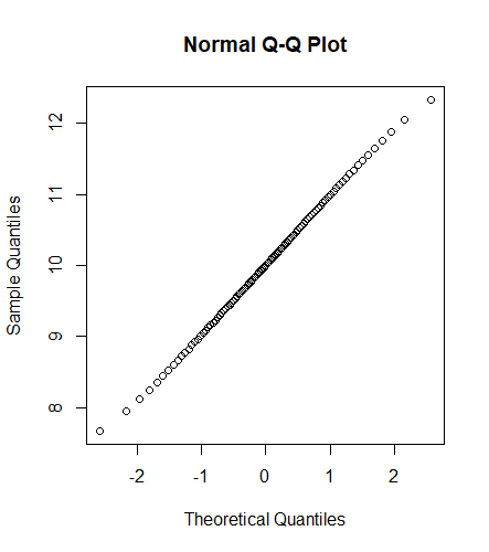
The Q-Q plot, also known as the quantile-quantile plot, is a graphical tool that helps us determine whether a set of data originated from a Normal or exponential distribution. For instance, if a statistical analysis assumes that residuals are normally distributed, a Normal Q-Q plot can be used to verify this assumption. This is merely a visual inspection and not a conclusive proof, so it is somewhat subjective. However, it enables us to see at a glance whether our assumption is plausible, and if not, how the assumption is violated and which data points contribute to the violation. A Q-Q plot is a scatterplot created by superimposing two quantile distributions. If both sets of quantiles came from the same distribution, the points should form a roughly straight line.

This post focuses primarily on introducing functions that can reproduce the Q-Q plot.

qqnorm is a generic function whose default method generates a standard QQ plot of the y values.

1
2
3
> # generate points from normal distribution
> x <- qnorm(seq(0.01,0.99,0.01))+10
> qqnorm(x)

hi

This can be reproduced using the function ppoints, which generates the sequence of probability points, as follows:

1
2
3
> # generate points from normal distribution
> x <- qnorm(seq(0.01,0.99,0.01))+10
> plot(x = qnorm(ppoints(length(x))),y = x)

qqplot could also reproduce the above

1
2
3
> # generate points from normal distribution
> x <- qnorm(seq(0.01,0.99,0.01))+10
> qqplot(x = qnorm(ppoints(length(x))),y = x)

qplot could also reproduce the above

1
2
3
> library(ggplot2)
> x <- qnorm(seq(0.01,0.99,0.01))+10
> qplot(x = qnorm(ppoints(length(x))),y = x)

For residual plot, however, we may choose to plot standardized residuals against theoretical quantiles in Q-Q plot.

We can use the R dataset randu as an illustration.

1
2
3
4
5
> str(randu)
'data.frame': 400 obs. of 3 variables:
$ x: num 0.000031 0.044495 0.82244 0.322291 0.393595 ...
$ y: num 0.000183 0.155732 0.873416 0.648545 0.826873 ...
$ z: num 0.000824 0.533939 0.838542 0.990648 0.418881 ...
  • If dependent variable is scaled, normal residual qqplot could be different
1
2
3
4
5
6
7
8
> model <- lm(z ~x+y, data = randu)
> var(resid(model))
[1] 0.07731478
> qqnorm(resid(model), main = 'normal qqplot when z is not scaled')

> model <- lm(10*z~x+y, data =randu)
> var(resid(model))
> qqnorm(resid(model), main = 'normal qqplot when z is scaled')

Clearly, scaling the dependent variable z affects the residual.

Before scaling

1
2
3
4
5
6
7
8
9
10
11
12
13
14
15
16
17
18
19
20
21
> model <- lm(z ~x+y,data = randu)
> summary(model)

Call:
lm(formula = z ~ x + y, data = randu)

Residuals:
Min 1Q Median 3Q Max
-0.51260 -0.23114 -0.01989 0.22893 0.56084

Coefficients:
Estimate Std. Error t value Pr(>|t|)
(Intercept) 0.48017 0.03811 12.598 <2e-16 ***
x 0.05424 0.04902 1.106 0.269
y -0.05713 0.04757 -1.201 0.230
---
Signif. codes: 0***0.001**0.01*0.05 ‘.’ 0.1 ‘ ’ 1

Residual standard error: 0.2788 on 397 degrees of freedom
Multiple R-squared: 0.007008, Adjusted R-squared: 0.002006
F-statistic: 1.401 on 2 and 397 DF, p-value: 0.2476

After scaling

1
2
3
4
5
6
7
8
9
10
11
12
13
14
15
16
17
18
19
20
21
> model <- lm(10*z~x+y,data =randu)
> summary(model)

Call:
lm(formula = 10 * z ~ x + y, data = randu)

Residuals:
Min 1Q Median 3Q Max
-5.1260 -2.3114 -0.1989 2.2893 5.6084

Coefficients:
Estimate Std. Error t value Pr(>|t|)
(Intercept) 4.8017 0.3811 12.598 <2e-16 ***
x 0.5424 0.4902 1.106 0.269
y -0.5713 0.4757 -1.201 0.230
---
Signif. codes: 0***0.001**0.01*0.05 ‘.’ 0.1 ‘ ’ 1

Residual standard error: 2.788 on 397 degrees of freedom
Multiple R-squared: 0.007008, Adjusted R-squared: 0.002006
F-statistic: 1.401 on 2 and 397 DF, p-value: 0.2476

Using standardized residuals, the expected value of the residuals is zero, while the variance is (approximately) one. This has two benefits:

  1. If you rescale one of your variables, the residual plots will not change.
  2. The residuals in the qqplot should lie on the line y = x
  3. The residuals in the qqplot should lie on the line y = x You anticipate that 95% of your residuals will fall between -1.96 and 1.96. This makes it simpler to identify outliers.
1
2
3
4
5
6
7
8
9
> model <- lm(z ~x+y,data = randu)
> var(rstandard(model))
[1] 1.002759
> qqnorm(rstandard(model),main = 'standardized residual qqplot before scaling')

> model <- lm(10*z~x+y,data =randu)
> var(rstandard(model))
[1] 1.002759
> qqnorm(rstandard(model), main = 'standardized residual qqplot after scaling')

Reference

This post mainly introduces how to build up a webpage from scratch using Hexo framework based on WSL system.

Install and configuration procedure

  • Install nvm

    $ curl -o- https://raw.githubusercontent.com/nvm-sh/nvm/v0.39.2/install.sh | bash

    Running either of the above commands downloads a script and runs it. The script clones the nvm repository to ~/.nvm, and attempts to add the source lines from the snippet below to the correct profile file (~/.bash_profile, ~/.zshrc, ~/.profile, or ~/.bashrc).

    1
    2
    export NVM_DIR="$([ -z "${XDG_CONFIG_HOME-}" ] && printf %s "${HOME}/.nvm" || printf %s "${XDG_CONFIG_HOME}/nvm")"
    [ -s "$NVM_DIR/nvm.sh" ] && \. "$NVM_DIR/nvm.sh" # This loads nvm

    On Linux, after running the install script, if you get nvm: command not found or see no feedback from your terminal after you type command -v nvm, simply close your current terminal, open a new terminal, and try verifying again. Alternatively, you can run the following commands for the different shells on the command line:

    bash: source ~/.bashrc

    zsh: source ~/.zshrc

    ksh: . ~/.profile

    These should pick up the nvm command.

  • Install hexo

    $ npm install -g hexo-cli

    Advanced users may prefer to install and use hexo package instead.

    1
    npm install hexo

    Once installed, you can run Hexo in two ways:

    1. npx hexo <command>
    2. Linux users can set relative path of node_modules/ folder:
    1
    echo 'PATH="$PATH:./node_modules/.bin"' >> ~/.profile

    then run Hexo using hexo <command>

  • Initialize webpage folder

    1
    2
    hexo init <webpage_name>
    cd <webpage_name>
  • Download configuration packages

    For example

    1
    2
    3
    4
    # Download local search toolkit
    npm install hexo-generator-searchdb
    # Download NEXT theme
    npm install hexo-theme-next

Troubleshooting

There is a strong possibility that we were created by an unknown entity or entities (I choose to switch between singular and plural for not knowing if there are a group of entities). Assuming this to be true, the following question can be posed: who creates the mysterious entity or entities that create us?

Following this line of reasoning, one would conclude that the entire universe is a simulation, functioning like Matryoshka dolls, and is replete with unending circulation.

hi

Given the notion that we are simulated with an extraordinarily high probability, emotions have lost their significance. In reality, the level of chemical compounds such as dopamine is closely connected with the degree of depression or happiness. However, not only feelings are pointless. According to this idea, intelligence, physical characteristics, and a variety of other factors are determined before birth.

From what I've seen, it's easy for people to accept that they're not strong or tall based on their genes and nutrition during adolescence, but it's often excruciatingly painful to accept that their fluid intelligence may not get better with time. To avoid depression, it would be advantageous to be a complete and absolute rationalist in the truest sense of the term, while at the same time accepting some dogmas.

hi

It is possible that we are modifiable modules. In this simulation experiment, the traits were allocated at the beginning of the birth, but the roads to our fate are countless. As a result, we could compare ourselves to humanoid robotics by employing various algorithms to traverse the final uncertainty. Bayes's rule might be used to determine the local optimal path, and reinforcement learning could be used to continuously adjust daily strategy.

This blog entry serves as a reminder to consider my weaknesses from the past to the present. Knowing every failure I've encountered, stupid decision I've made, and wrong verbal response or body language I've displayed has been the primary discipline in my life, and will remain so in the future.

Randomization, replication, repeated measurement, blocking

randomization means both the allocation of the experimental material and the order in which the individual runs of the experiment are to be performed randomly. Randomization could meet the requirement of the statistical methods that the observations (or errors) are independently distributed random variables. By using randomization, extraneous errors could be averaged out.

replication means an independent repeat run of each factor combination. First it allows the experimenter to obtain an estimate of the experimental error; this estimate of error becomes a basic unit of measurement for determining whether observed differences in the data are really statistically different. Second if the sample mean is used to estimate the true mean response for one of the factor levels in the experiment, replication permits the experimenter to obtain a more precise estimate of this parameter.

Repeated measurement involves measuring the same subject multiple times; Replication involves running the same study on different subjects with identical conditions (same factor combination)

Blocking is a design technique used to improve the precision with which comparisons among the factors of interest are made. Often blocking is used to reduce or eliminate the variability transmitted from nuisance factors, which may influence the experimental response but in which we are not directly interested.

standard deviation and standard error

  • Standard deviation describes variability within a single sample, while standard error describes variability across multiple samples of a population
  • Standard deviation is a descriptive statistic that can be calculated from sample data, while standard error is an inferential statistic that can only be estimated

Standard deviation involves population standard deviation \(\sigma\) and sample standard deviation \(s_n\). Sample standard deviation \(s_n\) includes biased estimator of \(\sigma\) as \(s_n=\sqrt{\frac{1}{n}\sum_i^n(x_i-\bar{x})^2}\) and unbiased estimator of \(\sigma\) as \(s_{n-1}=\sqrt{\frac{n}{n-1}s_n^2}=\sqrt{\frac{1}{n-1}\sum_{i=1}^n(x_i-\bar{x})^2}\)

Standard error is the standard deviation of the estimator \(\hat{\theta}\), and can be said as the standard deviation of the sampling distribution. Standard error of the mean \(\bar{x}\) (SEM) is equal to the population standard deviation divided by the square root of number of samples \(n\).

Suppose \(X_1,X_2,\cdots,X_n\) are a random sample from an \(N(\mu,\sigma^2)\) distribution. Then the standard deviation of \(\bar{X}\) is the standard error, as \(SD(\bar{X})=\sigma/\sqrt{n}\). Usually the \(\sigma\) is unknown, and is estimated by \(s_n\) or \(s_{n-1}\). Therefore, by giving the observed sample standard deviation \(s_n\) or \(s_{n-1}\), the standard error of the mean \(\bar{X}\) could be estimated by \(SE(\bar{X})=\frac{s_n}{\sqrt{n}}\) or \(SE(\bar{X})=\frac{s_{n-1}}{\sqrt{n}}\)

Confidence interval and credible interval

A great explanation of the difference between confidence interval and credible interval can be found in What's the difference between a confidence interval and a credible interval?

Sufficient statistic

Here is an useful Q&A explaining the definition of sufficient statistic

Understanding Sufficient statistic.

Power, sample size, and effect size

Here is a great blog explaining the definition of power, sample size calculation and effect size calculation

power and sample size determination

Reference

To Prove \(\bar{X}\) and \(X_i-\bar{X}\) are independent if \(X_i's\) are normally distributed and \(\bar{X}\) and \(X_i-\bar{X}\) are uncorrelated, two conditions are needed to be fulfilled:

  • Prove that given a joint MGF \(M_{X,Y}(s,t)\), \(M_{X,Y}(s,t)=M_X(s)\cdot M_Y(t)\) is the sufficient condition for independence of \(X\) and \(Y\)
  • Prove MGF of \((\bar{X},X_i-\bar{X})\) can be expressed as product of MGF of \(\bar{X}\) and MGF of \(X_i-\bar{X}\)

It's worth mentioning the uniqueness theorem of MGFS:

Theorem 1:

Suppose \(\exists\mathbf{t}>0\) such that \(M_{\mathbf{X}}(\mathbf{t})<\infty\) for all \(\mathbf{t}\in\mathbb{R}^n\) with \(||\mathbf{t}||\leq r\). Then, the distribution of \(\mathbf{X}\)

is determined uniquely by the function \(M_{\mathbf{X}}\). That is, if \(\mathbf{Y}\) is any random vector whose MGF is the same as \(M_{\mathbf{X}}\), then \(\mathbf{Y}\) has the same distribution as \(\mathbf{X}\)

Let \(\mathbf{X}\) be a random \(n-\)vector with a MGF that is finite in an open neighborhood of the origin \(0\in \mathbb{R}^n\). Let \(\tilde{X}\) denote an independent copy of \(\mathbf{X}\). Define a new random vector \(\mathbf{Y}\) as follows: \[ \mathbf{Y:=}\begin{bmatrix}X_1\\ \vdots \\ X_r\\\tilde{X}_{r+1}\\ \vdots\\ \tilde{X}_n\end{bmatrix} \] Then, \[ \begin{gather*} M_{\mathbf{Y}}(\mathbf{t})=Ee^{\sum_{i=1}^rt_iX_i}\cdot Ee^{\sum_{j=r+1}^nt_jX_j}\\ =M_{\mathbf{X}}(t_1,\cdots,t_r,0\cdots,0)\cdot M_{\mathbf{X}}(0,\cdots,0,t_{r+1},\cdots,t_n) \end{gather*} \] Suppose there exists \(r=1,\cdots,n\) such that \[ M_{\mathbf{X}}(\mathbf{t})=M_{\mathbf{X}}(t_1,\cdots,t_r,0,\cdots,0)\cdot M_{\mathbf{X}}(0,\cdots,0,t_{r+1},\cdots,t_n) \] for all \(\mathbf{t}\in \mathbb{R}^n\).

Then according to the theorem 1, \(\mathbf{X}\) and \(\mathbf{Y}\) have the same MGF’s, and therefore have the same distribution. That is, for all sets \(A_1,\cdots,A_n,\) there is \[ P\{X_1\in A_1,\cdots,X_n\in A_j\}=P\{Y_1\in A_1,\cdots,Y_n\in A_n\} \] which is, by construction equal to \[ P\{X_1\in A_1,\cdots,X_r\in A_r\}\cdot P\{\tilde{X}_{r+1}\in A_{r+1},\cdots,\tilde{X}_n\in A_n\} \] Since \(\tilde{X}\) has the same distribution as \(\mathbf{X}\), this proves that \[ P\{X_1\in A_1,\cdots, X_n\in A_n\}=P\{X_1\in A_1,\cdots,X_r\in A_r\}\cdot P\{X_{r+1}\in A_{r+1},\cdots,X_n\in A_n\} \] Which implies that \((X_1,\cdots,X_r)\) and \((X_{r+1},\cdots,X_n)\) are independent.

Then we have the second theorem

Theorem 2:

(Independence theorem of MGFs). Let \(X\) be a random n-vector with a MGF that is finite in an open neighborhood of the origin \(\mathbf{0}\in \mathbb{R}^n\). Suppose there exists \(r=1,\cdots,n\) such that \[ M_{\mathbf{X}}(\mathbf{t})=M_{\mathbf{X}}(t_1,\cdots,t_r,0,\cdots,0)\cdot M_{\mathbf{X}}(0,\cdots,0,X_{r+1},\cdots,X_n) \] for all \(\mathbf{t}\in\mathbb{R}^n\). Then \((X_1,\cdots,X_r)\) and \((X_{r+1},\cdots,X_n)\) are independent

By now, we have proved the first statement that

Given a joint MGF \(M_{X,Y}(s,t)\), \(M_{X,Y}(s,t)=M_X(s)\cdot M_Y(t)\) is the sufficient condition for independence of \(X\) and \(Y\)

Next we prove the second statement, by utilizing the first statement.

The proof process is given by the answer to my posted question Prove \(\bar{X}\) and \(X_i-\bar{X}\) are independent if \(X_i's\) are independently normally distributed

I hereby paste this elegant answer in my blog, and also give thanks to Damian Pavlyshyn

(Note: In this answer I'll only consider standard normal \(X_i\)s, since it's no harder to do when they have other means and variances)

One way of doing this is with moment generating functions. For a bivariate random variable \(Z = (Z_1, Z_2)\), \(Z_1\) and \(Z_2\) are independent if and only if the moment generating function \(M_Z(\mathbf{s}) = \mathbf{E} e^{\mathbf{s}^T Z}\) factors into a product of a functions of \(s_1\) and \(s_2\) only, where \(\mathbf{s} = (s_1, s_2)\).

Now, the thing to notice is that \((\bar{X}, X_i - \bar{X})\) is a linear transformation of the whole sample \(X = (X_1, \dotsc, X_n)\). Namely, \[ \begin{pmatrix}\bar{X} \\ X_i - \bar{X}\end{pmatrix} = \begin{pmatrix}\mathbf{1}^T/n \\ e_i^T - \mathbf{1}^T/n\end{pmatrix} X := H X \] where \(\mathbf{1}\) is a vector of all \(1\)s and \(e_i\) is the vector of all \(0\)s with a \(1\) in the \(i\)th entry.

We can use this to write down the MGF: \[ \begin{align*} \mathbf{E} \exp\biggl\{\mathbf{s}^T \begin{pmatrix}\bar{X} \\ X_i - \bar{X}\end{pmatrix}\biggr\} = \mathbf{E} \exp\{\mathbf{s}^T H X\} = \mathbf{E} \exp\{(H^T\mathbf{s})^T X\} \end{align*} \] Then we can use the known moment generating function of a vector of iid normals (\(\mathbf{E} e^{\mathbf{t}^T X} = \exp\{\frac{1}{2}\mathbf{t}^T \mathbf{t}\}\)) to conclude that \[ \mathbf{E} \exp\{(H^T\mathbf{s})^T X\} = \exp\{\frac{1}{2}(H^T\mathbf{s})^T(H^T\mathbf{s})\} = \exp\{\frac{1}{2}\mathbf{s}^T HH^T \mathbf{s}\}. \]

Now, we can multiply \[ \begin{gather*} HH^T = \begin{pmatrix}\mathbf{1}^T/n \\ e_i^T - \mathbf{1}^T/n\end{pmatrix} \begin{pmatrix}\mathbf{1}/n , & e_i - \mathbf{1}/n\end{pmatrix} \\ = \begin{pmatrix} \mathbf{1}^T/n \mathbf{1}/n & \mathbf{1}^T/n (e_i - \mathbf{1}/n) \\ (e_i - \mathbf{1}/n)^T \mathbf{1}/n & (e_i - \mathbf{1}/n)^T(e_i - \mathbf{1}/n) \end{pmatrix} \\ = \begin{pmatrix} 1/n & 0 \\ 0 & 1 - 1/n \end{pmatrix} \end{gather*} \]

so that the MGF becomes \[ \exp\biggl\{\frac{1}{2}\mathbf{s}^T HH^T \mathbf{s}\biggr\} = \exp\biggl\{\frac{1}{2}\biggl(\frac{1}{n}s_1^2 + \frac{n-1}{n}s_2^2\biggr)\biggr\} = e^{\frac{1}{2n}s_1^2} e^{\frac{n-1}{2n} s_2^2}. \]

Since this factors into terms containing only \(s_1\) and \(s_2\) respectively, we conclude that \(\bar{X}\) and \(X_i - \bar{X}\) are independent (and also that they have \(N(0, 1/n)\) and \(N(0, 1 - 1/n)\) distributions respectively).

Reference
8 Imperatives for Good project Management and Delivery

graph TB
A[Set expectations] --> B[Make projects as small as possible]
B --> C[Isolate the unknown from the known]
C --> D[Manage from the end backward]
D --> E[Have everything in writing]
E --> F[Deal with everthing as early as possible]
F --> G[Verify you have met all requirements]
G --> H[Measure and analyze yourself]

Reference

FTC homepage

FTC 2021 Webinar Series Talk 1: Michael Hamada - On Reading Youden

FTC 2021 Webinar Series Talk 2: Nathaniel Stevens - Probability of Agreement

FTC 2021 Webinar Series Talk 3: Wendy Martinez - The Importance of Data Ethics

FTC 2021 Webinar Series Talk 4: Roshan Joseph - MaxPro Designs for Computer Experiments

FTC 2021 Webinar Series Talk 5: Christine Anderson-Cook - Statistical Innovation

FTC 2021 Webinar Series Talk 6: Nachtsheim, Eck, and Albrecht - DOE for Dimensional Analysis

FTC 2021 Webinar Series Talk 7: Brad Jones - The Joy of Collaboration

FTC 2021 Webinar Series Talk 8: Jon Stallrich - Optimal EMG Sensor Placement for Robot Prosthetics

FTC 2021 Webinar Series Talk 9: Tony Pourmohamad - Stat Filter Approach to Constrained Optimization

  • Allow multiple results during one execution for one cell
1
2
from IPython.core.interactiveshell import InteractiveShell
InteractiveShell.ast_node_interactivity = "all"
  • Tell python interpreter to read code based on utf-8
1
2
#!/usr/bin/env python3
# -*- coding: utf-8 -*-