Count unique words

Posted on 2022-06-12 Edited on 2022-11-07 In R

Below is some R code that could be employed to summarize the unique words from the text.

words <- read.table(file.choose(), header = FALSE,fill = TRUE) # import txt file

words <- apply(words,c(1,2),function(x) gsub("[[:punct:]]", "", x)) # remove all special characters

words <- words[(words !='') ] # remove all NA content

x_numbers <- unlist(regmatches(words, gregexpr("[[:digit:]]+", words))) # extract numbers from string

words <- gsub('[[:digit:]]+', '', words) # remove all content containing numbers

words <- words[(words !='') ] # remove all NA content

x_numbers <- unlist(regmatches(words, gregexpr("[[:digit:]]+", words))) # extract numbers from string

length(unique(words)) # count unique words

shell command

Posted on 2022-06-11 Edited on 2022-11-07 In Linux

Command to the ~./bash_logout so that the history will get cleared when you logout

1	echo `history -c` >> ~/.bash_logout

Get the name of the history file

1	echo "$HISTFILE"

See the current history

1 2	history history \| grep 'du'

Hide and display the cursor in the shell

# Hide the cursor
echo -e "\033[?25l"

# Display the cursor
echo -e "\033[?25h"

Three ways of multiple line annotation

:<<EOF
annotation text...
annotation text...
annotation text...
EOF

:<<'
annotation text...
annotation text...
annotation text...
'

:<<!
annotation text...
annotation text...
annotation text...
!

Make file executable

1	chmod +x <file.name>

Use math equation in shell script (example)

#!/bin/bash

val=`expr 2 + 2`
echo "sum of two numbers: $val"

Operators in shell script

Enable interpretation of the backslash escapes

echo -e

Read varable and assign to a variable <variable.name>

1	read <variable.name>

vi/vim language and affiliated shortcuts

Shell I/O redirection

Reference

sum of normal random variables

Posted on 2022-06-08 Edited on 2022-11-07 In Mathematics

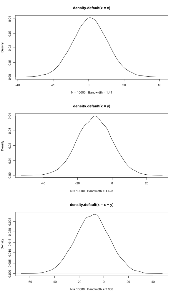
Suppose $X,Y$ are independent random variables from normal distributions, then sum of these two random variables is also a normal random variable. The proof of this statement could be referred to

Wikipedia-Proof using convolutions

We could also generate graphs to elucidate this process

> x <- rnorm(10000,1,10)
> y <- rnorm(10000,-10,10)
> par(mfrow = c(3,1))
> plot(density(x))
> plot(density(y))
> plot(density(x+y))

Reference

lnE(X) and E(lnX)

Posted on 2022-06-08 Edited on 2022-11-07 In Mathematics

Since $lnx$ is the concave function, by Jensen's inequality, we know that \[ ln[E(X)]>E[lnX] \] Another proof can be displayed as follows:

From Simplest or nicest proof that $1+x \le e^x$, we can prove that

\[ e^x\geq 1+x \]

Expectation of $e^x$ is \[ \begin{gather*} E(e^Y)=e^{E(Y)}E(e^{Y-E(Y)})\\ \geq e^{EY}E(1+Y-EY)\\ =e^{EY} \end{gather*} \] Therefore, we have \[ e^{EY}\leq E[e^Y] \] Denote $Y=lnX$, we have \[ e^{ElnX}\leq E(e^{lnX})=EX\\ \Rightarrow E(lnX)\geq ln(EX) \] The equality holds if and only if $X$ is almost surely constant.

Reference

E(X)/E(Y) and E(X/Y)

Posted on 2022-06-07 Edited on 2022-11-07 In Mathematics

In this part we aim to discover the relationship between $E[\frac{X}{Y}]$ and $\frac{EX}{EY}$ under the assumption that

$X,Y$ are independent

Since $X,Y$ are independent, then \[ \begin{gather*} P(X\leq x, \frac{1}{Y}\leq y)\\ =P(X\leq x, Y\geq \frac{1}{y})\\ =P(X\leq x)P(Y\geq \frac{1}{y})\\ =P(X\leq x)P(\frac{1}{Y}\leq y)\\ \end{gather*} \] We know that event $A,B$ are independent if and only if $P(A,B)=P(A)P(B)$;

Thus $X,\frac{1}{Y}$ are independent. This implies that \[ E[\frac{X}{Y}]=E(X)E(\frac{1}{Y}) \] Assume $E[X],E[\frac{1}{Y}]$ are finite.

The function $\frac{1}{y}$ is strictly convex over the domain $y>0$. So if $Y>0$ with prob $1$, then by Jensen's inequality we have: \[ E[\frac{1}{Y}]\geq\frac{1}{E[Y]} \] with equality if and only if $Var(Y)=0$ which is when $Y$ is a constant.

Thus if $X,Y$ are indepenent and if $Y>0$ with prob $1$ then

$E[X]=0\Rightarrow E[\frac{X}{Y}]=0=\frac{EX}{EY}$
$E[X]>0\Rightarrow E[\frac{X}{Y}]\geq \frac{EX}{EY}$ with equality if and only if $Var(Y)=0$
$E[X]<0\Rightarrow E[\frac{X}{Y}]\leq \frac{EX}{EY}$ with equality if and only if $Var(Y)=0$

Reference

$E(X)/E(Y)$ compared to $E(X/Y)$

Uncorrelated vs independent

Posted on 2022-06-07 Edited on 2022-11-07 In statistics

Uncorrelation means there is no linear dependence between the two random variables, while independence means no types of dependence exist between the two random variables.

Uncorrelated random variables may not be independent, but independent random variables must be uncorrelated.

For example, $Z\sim N(0,1),X=Z,Y=Z^2$ \[ \begin{gather*} Cov(X,Y)=E[XY]-E[X]E[Y]\\ =E[Z^3]-E[Z]E[Z^2]\\ =E[Z^3]-0\\ =E[Z^3] \end{gather*} \] The moment generating function of distribution of $Z$ is \[ \begin{gather*} M_Z(t)=E[e^{tz}]\\ =\int e^{tx}\frac{1}{\sqrt{2\pi}}e^{-\frac{z^2}{2}}dz\\ =\int \frac{1}{\sqrt{2\pi}}e^{-\frac{1}{2}(z^2-2tz)}dz\\ =\int \frac{1}{\sqrt{2\pi}}e^{-\frac{1}{2}(z^2-2tz+t^2)+\frac{1}{2}t^2}dz\\ =\int \frac{1}{\sqrt{2\pi}}e^{-\frac{1}{2}(z-t)^2+\frac{1}{2}t^2}dz\\ =e^{\frac{1}{2}t^2}\int\frac{1}{\sqrt{2\pi}}e^{-\frac{1}{2}(z-t)^2}dz\\ =e^{\frac{1}{2}t^2} \end{gather*} \] Using the mgf we obtain the $E[Z^3]$ as \[ \begin{gather*} E[Z^3]=M_Z'''(t=0)\\ =(0)e^{\frac{1}{2}(0)^2}+2(0)e^{\frac{1}{2}(0)^2}+(0)^3e^{\frac{1}{2}(0)^2}=0 \end{gather*} \] Therefore \[ Cov(X,Y)=E[Z^3]=0 \] This implies $X,Y$ are uncorrelated, but they are dependent

Reference

Jensen's inequality

Posted on 2022-06-06 Edited on 2022-11-07 In Mathematics

The expression of variance \[ Var(X)=E[(X-EX)^2]=EX^2-(EX)^2\geq 0 \] Implies that \[ EX^2\geq (EX)^2 \] Here $X^2$ is an example of the convex function. The definition of convex function is

A twice-differentiable function $g:I\rightarrow \mathbb{R}$ is convex if and only if $g''(x)\geq 0$ for all $x\in I$

Below is a typical example of the convex function. The function is convex if the line segment between two points from the curve lies above the curve. On the other hand, if the line segment aloways lies below the curve, then the function is said to be concave.

The Jensen's inequality states that for any convex function $g$, we have $E[g(X)]\geq g(E(X))$. To be specific.

If $g(x)$ is a convex function on $R_X$, and $E[g(X)]$ and $g[E(X)]$ are finite, then \[ E[g(X)]\geq g[E(X)] \]

Reference

Jensen's Inequality

delta method

Posted on 2022-06-02 Edited on 2022-11-07 In statistics

The Taylor series of a real or complex-valued function f (x) that is infinitely differentiable at a real or complex number $a$ is the power series \[ f(x)\approx f(a)+\frac{f'(a)}{1}(x-a)+\frac{f''(a)}{2!}(x-a)^2+\frac{f'''(a)}{3!}(x-a)^3+\cdots \] Where $n!$ denotes the factorial of $n$. In the more compact sigma notation, this can be written as \[ \underset{n=0}{\overset{\infty}{\sum}}\frac{f^{(n)}(a)}{n!}(x-a)^n \] The property of taylor series determines two things:

The approximation would be more closer to the original value of $f(x)$ if we add more terms
As $x$ is more closer to the $a$, the approximation will be more accurate

We provide the following example to illustrate above two properties \[ \begin{gather*} f(x)=lnx(x\in(0,1))\\ f(x)\approx lnx_0+(x-x_0)\frac{1}{x_0}(\text{first order})\\ f(x)\approx lnx_0+(x-x_0)\frac{1}{x_0}-\frac{1}{2}(x-x_0)^2\frac{1}{x_0^2}(\text{second order}) \end{gather*} \]

c1 <- curve(log(x))
c2 <- curve(log(0.5)+2*(x-0.5))
plot(curve(log(0.5)+2*(x-0.5)-0.5*(x-0.5)^2*4),
     col = 'red',type = 'l',xlab = 'x',ylab = 'y',
     ylim = c(-3,0),main = 'Taylor approximation for lnx at point 0.5')
lines(c1$x,c1$y,col = 'green')
lines(c2$x,c2$y,col = 'blue')
legend('topleft',
       c('lnx','first order','second order'),
       inset = 0.001,
       cex = 0.5,
       lty = c(1,1),
       col = c('green','blue','red'))

Below is a good tip for explaining the delta method, from (Alan. H. Feiveson, NASA)

The delta method, in its essence, expands a function of a random variable about its mean, usually with a one-step Taylor approximation, and then takes the variance. For example, if we want to approximate the variance of $f(X)$ where $X$ is a random variable with mean $\mu$ and $f()$ is differentiable, we can try \[ f(x)=f(\mu)+(x-\mu)f'(\mu) \] so that \[ \begin{gather*} var[f(X)]=var(f(\mu)+(X-\mu)f'(\mu))\\ =var(X-\mu)[f'(\mu)]^2\\ =var(X)[f'(\mu)]^2 \end{gather*} \] This is a good approximation only if $X$ has a high probability of being close enough to its mean($\mu$) so that the Taylor approximation is still good.

Reference

Use of log in likelihood

Posted on 2022-05-29 Edited on 2022-12-20 In statistics

Below is an interesting question about likelihood from a thread in quora

Why do we always put log() in Maximum likelihood estimation before estimate the parameter?

The answer to this question is

$log(x)$ is an increasing function. Therefore solving the following two problems gives the same result: \[ \begin{gather*} \underset{\theta}{max}\ f(x;\theta)\\ \underset{\theta}{max}\ log(f(x;\theta)) \end{gather*} \]

From above two equations, it seems there is no necessity to put log to solve the problem. The reason to put log is because most of the times it's faster to deal with sums than the products in the objective since it is more convenient to differentiate the sums than produces. For example, suppose we have $n$ data points $x_1,x_2,\cdots,x_n$ which are iid drawn from $f(x;\theta)$ with unknown $\theta$. MLE of $\theta$ will solve the following problems:

\[ \begin{gather*} \underset{\theta}{max}\ \underset{i=1}{\overset{n}{\prod}}f(x_i;\theta)\\ \underset{\theta}{max}\ \underset{i=1}{\overset{n}{\sum}}log(f(x_i;\theta)) \end{gather*} \]

Two equations are equivalent, but it may take few additional steps to reach the same condition if we use the product

Reference

Why do we always put log() in Maximum Likelihood estimation before estimate the parameter?

Laplace approximation

Posted on 2022-05-29 Edited on 2022-11-07 In statistics

The Laplace technique can be used to approximate the reasonably well behaved functions that have most of their mass concentrated in a small area of their domain.(Laplace approximation) Technically, it works for functions that are in the class of $\mathcal{L}^2$, which is also called the square integrable function, meaning \[ \int g(x)^2dx <\infty \] Such a function generally has a very rapid decreasing tails so that in the far reaches of the domain we would not expect to see large spikes.

The Laplace approximation framework is a simple but widely used framework, and aims to find a Gaussian approximation to a probability density defined over a set of continuous variables. (Laplace approximation)

In Bayesian statistics, Laplace approximation can refer to either approximating the posterior normalizing constant with Laplace's method or approximating the posterior distribution with a Gaussian centered at the maximum a posteriori estimate.(Amaral Turkman 2019)

Suppose we want to approximate the pdf $p(\theta)$, which doesn't belong to any known distribution. The density curve is smooth and well peaked around its point of maxima $\hat{\theta}$. Thereby, $\frac{dp(\theta)}{d\theta}|_{\hat{\theta}}=0$ and $\frac{d^2p(\theta)}{d\theta^2}|_{\hat{\theta}}<0$; thus we can conclude that $\frac{dlnp(\theta)}{d\theta}|_{\hat{\theta}}=0$ and $\frac{d^2lnp(\theta)}{d\theta^2}|_{\hat{\theta}}<0$

Then we can approximate it by a normal pdf. Denote $h(\theta)=lnp(\theta)$ \[ \begin{gather*} h(\theta)\approx lnp(\hat{\theta})+(\theta-\hat{\theta})\frac{dlnp(\theta)}{d\theta}|_{\hat{\theta}}+\frac{1}{2}(\theta-\hat{\theta})^2\frac{d^2lnp(\theta)}{d\theta^2}|_{\hat{\theta}}\\ =lnp(\hat{\theta})-\frac{1}{2}(\theta-\hat{\theta})^2\frac{-d^2lnp(\theta)}{d\theta^2}|_{\hat{\theta}}\ (\frac{dlnp(\theta)}{d\theta}|_{\hat{\theta}}=0)\\ =lnp(\hat{\theta})-\frac{(\theta-\hat{\theta})^2}{2\sigma^2}\ (\sigma^2=(\frac{-d^2lnp(\theta)}{d\theta^2}|_{\hat{\theta}})^{-1}>0)\\ \Rightarrow p(\theta)=e^{h(\theta)}\approx p(\hat{\theta})e^{-\frac{(\theta-\hat{\theta})^2}{2\sigma^2}}\\ \Rightarrow p(\theta)\propto e^{-\frac{(\theta-\hat{\theta})^2}{2\sigma^2}} \end{gather*} \] Suppose $f(\theta)=e^{-\frac{(\theta-\hat{\theta})^2}{2\sigma^2}}$, then we can approximate $p(\theta)$ as \[ \begin{gather*} p(\theta)\approx \frac{1}{\int f(\theta)d\theta}f(\theta)\\ =\frac{1}{\sqrt{2\pi}\sigma\int \frac{1}{\sqrt{2\pi}\sigma}e^{-\frac{(\theta-\hat{\theta})^2}{2\sigma^2}}d\theta}e^{-\frac{(\theta-\hat{\theta})^2}{2\sigma^2}}\\ =\frac{1}{\sqrt{2\pi}\sigma}e^{-\frac{(\theta-\hat{\theta})^2}{2\sigma^2}}\\ \text{where }\int f(\theta)d\theta\text{ is the normalizing term} \end{gather*} \] As a result, pdf of $\theta$ is approximated by a normal distribution using Laplace method, which can be shown as below \[ \begin{gather*} \theta\sim N(\hat{\theta},\sigma^2)\\ \sigma^2=(\frac{-d^2lnp(\theta)}{d\theta^2}|_{\hat{\theta}})^{-1}>0 \end{gather*} \]